The Relation Between Runs and Wins

Learning objectives:

Introduce sabermetrics
Establish Pythagorean win-loss
Implement linear regression models

library("abdwr3edata")
library("ggrepel")
library("gt")
library("Lahman")
library("tidyverse")

crcblue <- "#2905A1"

Session Info

sessionInfo()

R version 4.4.2 (2024-10-31 ucrt)
Platform: x86_64-w64-mingw32/x64
Running under: Windows 10 x64 (build 19045)

Matrix products: default


locale:
[1] LC_COLLATE=English_United States.utf8 
[2] LC_CTYPE=English_United States.utf8   
[3] LC_MONETARY=English_United States.utf8
[4] LC_NUMERIC=C                          
[5] LC_TIME=English_United States.utf8    

time zone: America/New_York
tzcode source: internal

attached base packages:
[1] stats     graphics  grDevices utils     datasets  methods   base     

other attached packages:
 [1] lubridate_1.9.4   forcats_1.0.0     stringr_1.5.1     dplyr_1.1.4      
 [5] purrr_1.0.4       readr_2.1.5       tidyr_1.3.1       tibble_3.2.1     
 [9] tidyverse_2.0.0   Lahman_12.0-0     gt_0.11.1         ggrepel_0.9.6    
[13] ggplot2_3.5.2     abdwr3edata_0.0.3

loaded via a namespace (and not attached):
 [1] generics_0.1.3     xml2_1.3.8         stringi_1.8.4      hms_1.1.3         
 [5] digest_0.6.37      magrittr_2.0.3     evaluate_1.0.3     grid_4.4.2        
 [9] timechange_0.3.0   RColorBrewer_1.1-3 fastmap_1.2.0      jsonlite_1.8.9    
[13] promises_1.3.2     scales_1.4.0       cli_3.6.3          shiny_1.10.0      
[17] rlang_1.1.5        withr_3.0.2        tools_4.4.2        tzdb_0.5.0        
[21] httpuv_1.6.15      vctrs_0.6.5        R6_2.6.1           mime_0.12         
[25] lifecycle_1.0.4    htmlwidgets_1.6.4  pkgconfig_2.0.3    pillar_1.10.2     
[29] later_1.4.1        gtable_0.3.6       glue_1.8.0         Rcpp_1.0.12       
[33] xfun_0.52          tidyselect_1.2.1   rstudioapi_0.17.1  knitr_1.50        
[37] farver_2.1.2       xtable_1.8-4       htmltools_0.5.8.1  rmarkdown_2.29    
[41] compiler_4.4.2

Recency

Following the textbook’s lead, let us find the most recent data in the Lahman package.

Teams |>
  select(yearID, teamID, franchID, G, W, L, R, RA) |>
  slice_tail(n = 5)

  yearID teamID franchID   G  W  L   R  RA
1   2023    PIT      PIT 162 76 86 692 790
2   2023    SDN      SDP 162 82 80 752 648
3   2023    SFN      SFG 162 79 83 674 719
4   2023    SLN      STL 162 71 91 719 829
5   2023    WAS      WSN 162 71 91 700 845

Shortened Seasons

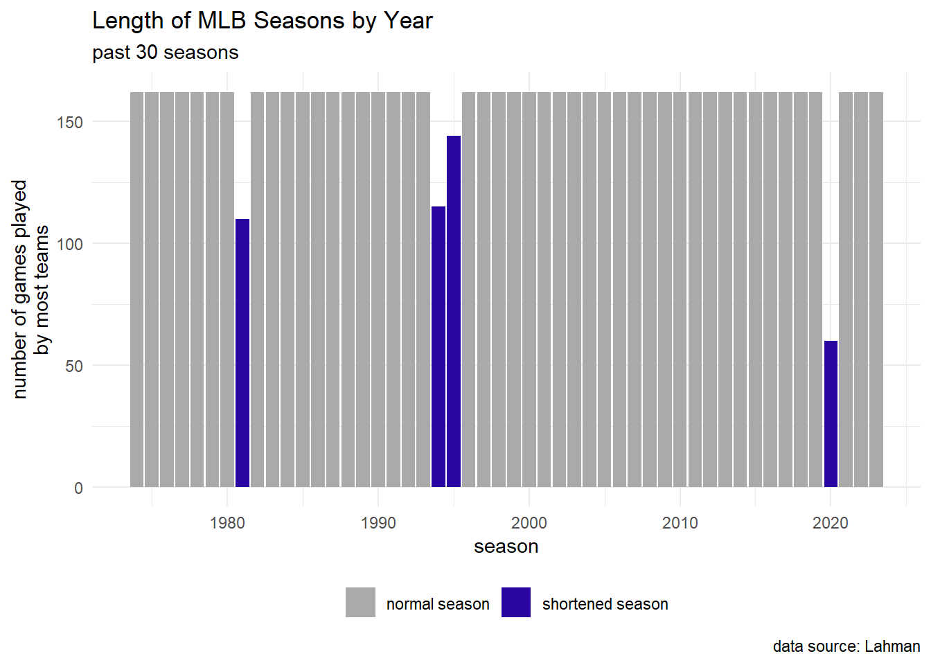
Some MLB seasons were shorter than others.

graph code

game_count_df <- Teams |>
  select(yearID, G) |>
  group_by(yearID, G) |>
  mutate(obs_count = n()) |>
  ungroup() |>
  distinct() |>
  
  # compute mode by year
  group_by(yearID) |>
  slice_max(order_by = obs_count, n = 1) |>
  ungroup()

game_count_df |>
  filter(yearID > 1973) |>
  mutate(season_bool = ifelse(G == 162, "normal season", "shortened season")) |>
  ggplot(aes(x = yearID, y = G)) +
  geom_bar(aes(fill = season_bool),
           stat = "identity") +
  labs(title = "Length of MLB Seasons by Year",
       subtitle = "past 30 seasons",
       caption = "data source: Lahman",
       x = "season",
       y = "number of games played\nby most teams") +
  scale_fill_manual(values = c("#AAAAAA", "#2905A1")) +
  theme_minimal() +
  theme(legend.position = "bottom",
        legend.title=element_blank())

1981: strike-shortened season
1994: strike-shortened season
1995: strike-shortened season
2000: pandemic-shortened season

Fun Fact!

According to Redditor u/pnabf

The Braves, who have 4 championships in their franchise history, have never won a WS when playing 162 games in a season

Let us check that!

Teams |>
  filter(franchID == "ATL") |>
  filter(WSWin == "Y") |>
  select(franchID, yearID, WSWin, G)

  franchID yearID WSWin   G
1      ATL   1914     Y 158
2      ATL   1957     Y 155
3      ATL   1995     Y 144
4      ATL   2021     Y 161

1995: strike-shortened season
2021: Sept 16 COL@ATL game was canceled due to rain

Rate Statistics

In baseball statistics, consider the use of both count statistics and rate statistics

count statistics (for example): $A B$ , $E R$ , $H$ , $I P$
rate statistics (for example):

$B A = \frac{H}{A B}, E R A = \frac{E R}{I P} \cdot 9$

Win Percentage

ch4_data <- Teams |>
  filter(yearID >= 1998, yearID != 2020) |>
  select(yearID, lgID, teamID, G, W, L, R, RA, DivWin, WCWin) |>
  
  # run differential
  mutate(RD = R - RA) |>
  
  # win percentage
  mutate(Wpct = W / (W + L)) |>
  
  # playoff win (Boolean)
  mutate(playoff_bool = ifelse(
    DivWin == "Y" | WCWin == "Y",
    "made playoffs", "missed playoffs"
  ))

Correlation

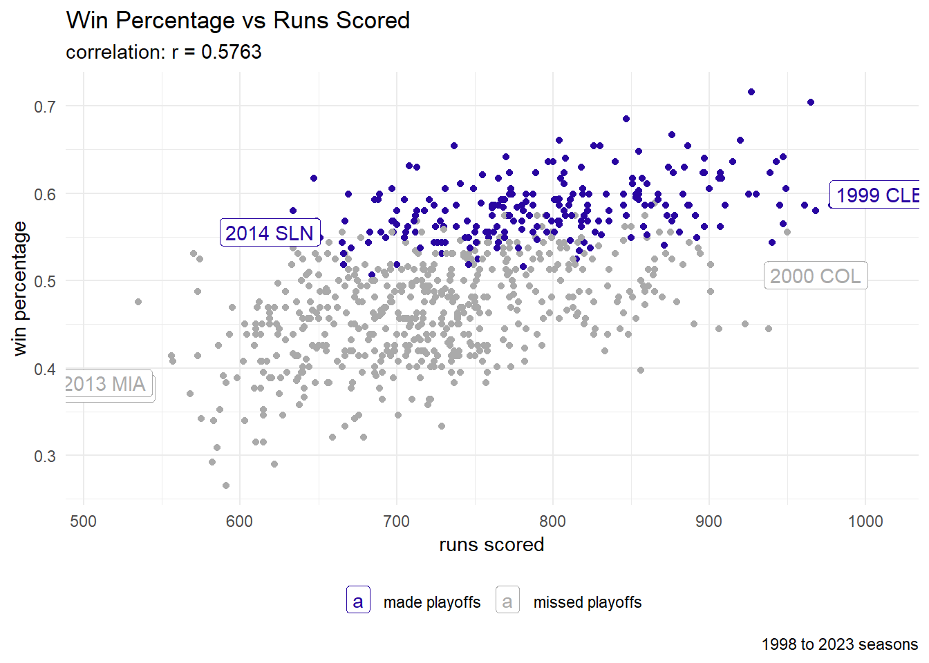
In short, we may want correlation values close to 1.0 or -1.0.

Offense

graph code

cor_value = cor(ch4_data$R, ch4_data$Wpct,
                use = "pairwise.complete.obs")

subset_for_labels <- ch4_data |>
  select(R, Wpct, playoff_bool, yearID, teamID) |>
  group_by(playoff_bool) |>
  mutate(highlight = ifelse(
    R == max(R) | R == min(R),
    1, 0
  )) |>
  ungroup() |>
  filter(highlight == 1) |>
  mutate(year_team = paste(yearID, teamID))

ch4_data |>
  ggplot(aes(x = R, y = Wpct)) +
  geom_point(aes(color = playoff_bool)) +
  geom_label(aes(x = R, y = Wpct, color = playoff_bool, label = year_team),
             data = subset_for_labels) +
  labs(title = "Win Percentage vs Runs Scored",
       subtitle = paste0("correlation: r = ", round(cor_value, 4)),
       caption = "1998 to 2023 seasons",
       x = "runs scored",
       y = "win percentage") +
  scale_color_manual(values = c("#2905A1", "#AAAAAA")) +
  theme_minimal() +
  theme(legend.position = "bottom",
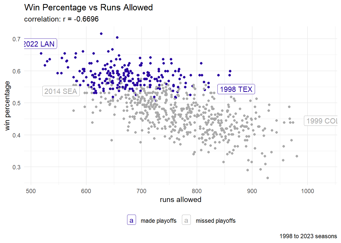
        legend.title=element_blank())

Defense

graph code

cor_value = cor(ch4_data$RA, ch4_data$Wpct,
                use = "pairwise.complete.obs")

subset_for_labels <- ch4_data |>
  select(RA, Wpct, playoff_bool, yearID, teamID) |>
  group_by(playoff_bool) |>
  mutate(highlight = ifelse(
    RA == max(RA) | RA == min(RA),
    1, 0
  )) |>
  ungroup() |>
  filter(highlight == 1) |>
  mutate(year_team = paste(yearID, teamID))

ch4_data |>
  ggplot(aes(x = RA, y = Wpct)) +
  geom_point(aes(color = playoff_bool)) +
  geom_label(aes(x = RA, y = Wpct, color = playoff_bool, label = year_team),
             data = subset_for_labels) +
  labs(title = "Win Percentage vs Runs Allowed",
       subtitle = paste0("correlation: r = ", round(cor_value, 4)),
       caption = "1998 to 2023 seasons",
       x = "runs allowed",
       y = "win percentage") +
  scale_color_manual(values = c("#2905A1", "#AAAAAA")) +
  theme_minimal() +
  theme(legend.position = "bottom",
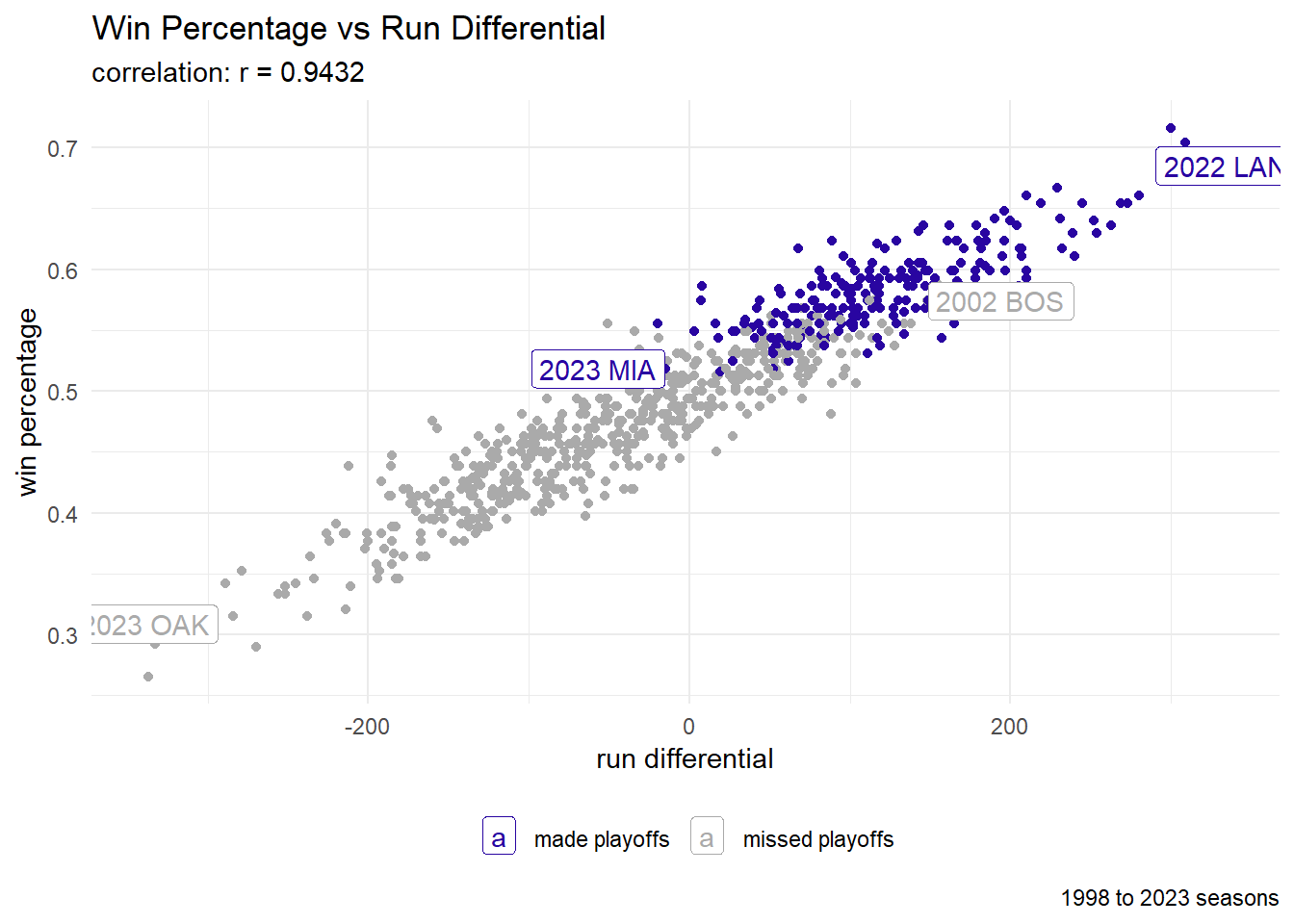
        legend.title=element_blank())

Run Differential

graph code

cor_value = cor(ch4_data$RD, ch4_data$Wpct,
                use = "pairwise.complete.obs")

subset_for_labels <- ch4_data |>
  select(RD, Wpct, playoff_bool, yearID, teamID) |>
  group_by(playoff_bool) |>
  mutate(highlight = ifelse(
    RD == max(RD) | RD == min(RD),
    1, 0
  )) |>
  ungroup() |>
  filter(highlight == 1) |>
  mutate(year_team = paste(yearID, teamID))

ch4_data |>
  ggplot(aes(x = RD, y = Wpct)) +
  geom_point(aes(color = playoff_bool)) +
  geom_label(aes(x = RD, y = Wpct, color = playoff_bool, label = year_team),
             data = subset_for_labels) +
  labs(title = "Win Percentage vs Run Differential",
       subtitle = paste0("correlation: r = ", round(cor_value, 4)),
       caption = "1998 to 2023 seasons",
       x = "run differential",
       y = "win percentage") +
  scale_color_manual(values = c("#2905A1", "#AAAAAA")) +
  theme_minimal() +
  theme(legend.position = "bottom",
        legend.title=element_blank())

Linear Regression

We will proceed by exploring a possible relationship between the run differential and the win percentage.

$W_{pct} = β_{0} + β_{1} * R D + ϵ$

In R, we make a linear model using the lm function.

lin_fit <- lm(Wpct ~ RD, data = ch4_data)
lin_fit #print coefficients


Call:
lm(formula = Wpct ~ RD, data = ch4_data)

Coefficients:
(Intercept)           RD  
  0.4999841    0.0006081

In ggplot2, we visualize the best-fit line using geom_smooth (with the method = 'lm' parameter).

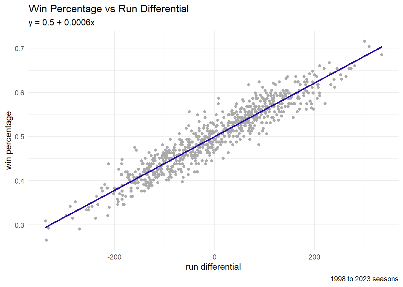
graph code

ch4_data |>
  ggplot(aes(x = RD, y = Wpct)) +
  geom_point(color = "#AAAAAA") +
  geom_smooth(color = "#2905A1",
              formula = "y ~ x",
              method = "lm",
              se = FALSE) +
  labs(title = "Win Percentage vs Run Differential",
       subtitle = "y = 0.5 + 0.0006x",
       caption = "1998 to 2023 seasons",
       x = "run differential",
       y = "win percentage") +
  theme_minimal() +
  theme(legend.position = "bottom",
        legend.title=element_blank())

$β_{0} = 0.5$

$R D = 0 \to W_{pct} = 0.5$
Over 162 games: 81 wins

$β_{1} = 0.0006$

$R D = + 10 \to W_{pct} = 0.506$
Over 162 games: 82 wins

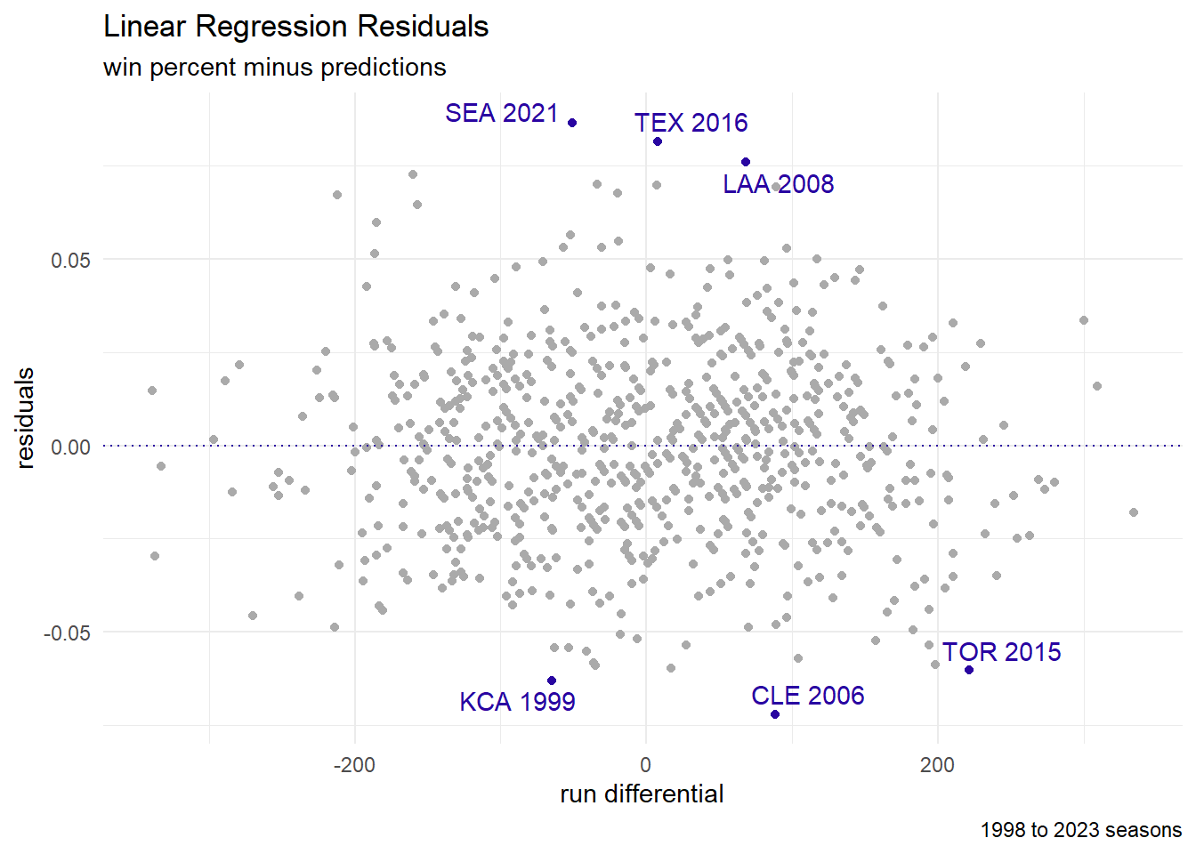
Residuals

Residuals are the differences between the predictions (aka fitted data) and the true values (aka response values).

ch4_data <- ch4_data |>
  mutate(preds = predict(lin_fit, newdata = ch4_data),
         resid = Wpct - preds)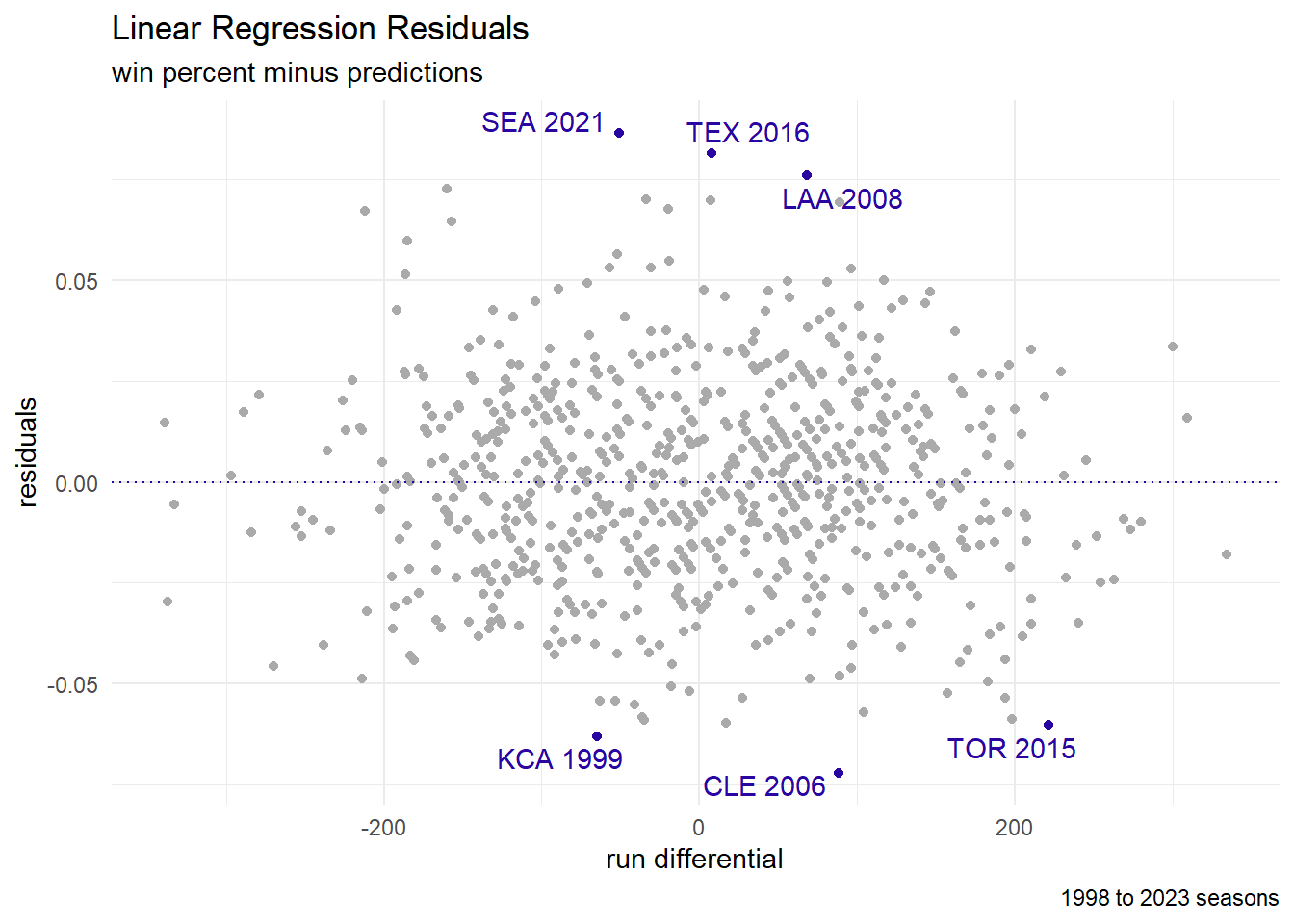

graph code

Residuals
top 3 and bottom 3
teamID	yearID	Wpct	preds	resid	desc
SEA	2021	0.56	0.47	0.09	performed better
TEX	2016	0.59	0.50	0.08	performed better
LAA	2008	0.62	0.54	0.08	performed better
TOR	2015	0.57	0.63	−0.06	performed worse
KCA	1999	0.40	0.46	−0.06	performed worse
CLE	2006	0.48	0.55	−0.07	performed worse

table code

oddities |>
  select(teamID, yearID, Wpct, preds, resid) |>
  mutate(desc = ifelse(resid > 0, "performed better", "performed worse")) |>
  gt() |>
  cols_align(align = "center") |>
  fmt_number(columns = c(Wpct, preds, resid),
             decimals = 2) |>
  tab_header(title = "Residuals",
             subtitle = "top 3 and bottom 3")

Balance

For linear models (through least-squares optimization), the average of the residuals should be zero:

mean(ch4_data$resid)

[1] 4.420171e-16

RMSE

The root mean square error acts similarly to a standard deviation to help measure along the variation of our data.

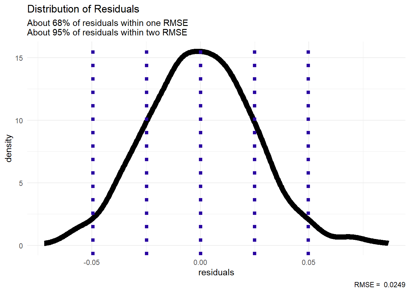
graph code

rmse <- sqrt(mean(ch4_data$resid^2))

ch4_data |>
  ggplot(aes(x = resid)) +
  geom_density(linewidth = 3) +
  geom_vline(color = "#2905A1",
             linetype = 3,
             linewidth = 2,
             xintercept = c(-2*rmse, -1*rmse, 0, rmse, 2*rmse)) +
  labs(title = "Distribution of Residuals",
       subtitle = "About 68% of residuals are within one RMSE\nAbout 95% of residuals are within two RMSE",
       caption = paste("RMSE = ", round(rmse, 4)),
       x = "residuals") +
  theme_minimal()

Discussion

What about extreme performances?
Should we relate count statistics to a rate statistic?
Can we make predictions during the season?

Pythagorean Formula

Bill James, regarded as the godfather of sabermetrics, empirically derived the following non-linear formula to estimate winning percentage, called the Pythagorean expectation.

$\hat{W_{pct}} = \frac{R^{2}}{R^{2} + R A^{2}}$

ch4_data <- ch4_data |>
  mutate(Wpct_pyt = R^2 / (R^2 + RA^2),
         resid_pyt = Wpct - Wpct_pyt)

# RMSE with exponent of 2
sqrt(mean(ch4_data$resid_pyt^2))

[1] 0.02570405

What should the exponent be?

$\frac{W}{W + L} = W_{pct} \approx \hat{W_{pct}} = \frac{R^{k}}{R^{k} + R A^{k}}$

algebra

$\begin{array}{rcl} \frac{W}{W + L} = W_{pct} & \approx & \hat{W_{pct}} = \frac{R^{k}}{R^{k} + R A^{k}} \\ \frac{W}{W + L} & \approx & \frac{R^{k}}{R^{k} + R A^{k}} \\ W R^{k} + W R A^{k} & \approx & W R^{k} + L R^{k} \\ W R A^{k} & \approx & L R^{k} \\ \frac{W}{L} \cdot R A^{k} & \approx & R^{k} \\ \frac{W}{L} & \approx & \frac{R^{k}}{R A^{k}} \\ \frac{W}{L} & \approx & {(\frac{R}{R A})}^{k} \\ \ln \frac{W}{L} & \approx & \ln {(\frac{R}{R A})}^{k} \end{array}$

$\ln \frac{W}{L} \approx k \ln (\frac{R}{R A})$

ch4_data <- ch4_data |>
  mutate(logWratio = log(W/L),
         logRratio = log(R/RA))
pyt_fit <- lm(logWratio ~ 0 + logRratio, data = ch4_data)
pyt_fit$coefficients

logRratio 
 1.834988

ch4_data <- ch4_data |>
  mutate(Wpct_pyt = R^1.835 / (R^1.835 + RA^1.835),
         resid_pyt = Wpct - Wpct_pyt)

# RMSE with exponent of 1.835
sqrt(mean(ch4_data$resid_pyt^2))

[1] 0.02494779

Luck

We can find the expected number of wins for a full season by multiplying the estimated win percentage (from the Pythagorean formula with an exponent of 1.835) by 162 games.

2011 Season
Performance vs Pythag Expectation
teamID	W	W_pyt	playoff_bool	diff	desc
DET	95	88.5	made playoffs	6.5	lucky
SFN	86	80.0	missed playoffs	6.0	lucky
MIL	96	90.1	made playoffs	5.9	lucky
ARI	94	88.3	made playoffs	5.7	lucky
CLE	80	75.3	missed playoffs	4.7	lucky
ATL	89	85.3	missed playoffs	3.7	lucky
CHA	79	75.3	missed playoffs	3.7	lucky
PIT	72	69.6	missed playoffs	2.4	lucky
BAL	69	66.7	missed playoffs	2.3	lucky
SLN	90	88.1	made playoffs	1.9	lucky
TOR	81	79.2	missed playoffs	1.8	lucky
WAS	80	78.8	missed playoffs	1.2	lucky
LAA	86	84.9	missed playoffs	1.1	lucky
MIN	63	61.9	missed playoffs	1.1	lucky
CHN	71	70.3	missed playoffs	0.7	lucky
SEA	67	66.7	missed playoffs	0.3	lucky
FLO	72	72.4	missed playoffs	−0.4	unlucky
TBA	91	91.4	made playoffs	−0.4	unlucky
PHI	102	102.6	made playoffs	−0.6	unlucky
NYN	77	78.6	missed playoffs	−1.6	unlucky
TEX	96	98.1	made playoffs	−2.1	unlucky
LAN	82	84.8	missed playoffs	−2.8	unlucky
OAK	74	77.2	missed playoffs	−3.2	unlucky
CIN	79	82.5	missed playoffs	−3.5	unlucky
BOS	90	93.7	missed playoffs	−3.7	unlucky
COL	73	77.2	missed playoffs	−4.2	unlucky
NYA	97	101.2	made playoffs	−4.2	unlucky
HOU	56	62.2	missed playoffs	−6.2	unlucky
KCA	71	77.8	missed playoffs	−6.8	unlucky
SDN	71	78.8	missed playoffs	−7.8	unlucky

table code

ch4_data |>
  filter(yearID == 2011) |>
  mutate(W_pyt = Wpct_pyt*162) |>
  select(teamID, W, W_pyt, playoff_bool) |>
  mutate(diff = W - W_pyt) |>
  mutate(desc = ifelse(diff > 0,
                       "lucky", "unlucky")) |>
  arrange(desc(diff)) |>
  gt() |>
  cols_align(align = "center") |>
  data_color(columns = diff,
             palette = "viridis") |>
  data_color(columns = playoff_bool,
             palette = "viridis",
             reverse = TRUE) |>
  fmt_number(columns = c(W_pyt, diff),
             decimals = 1) |>
  tab_header(title = "2011 Season",
             subtitle = "Performance vs Pythag Expectation")

2023 Season
Performance vs Pythag Expectation
teamID	W	W_pyt	playoff_bool	diff	desc
MIA	84	74.9	made playoffs	9.1	lucky
BAL	101	93.8	made playoffs	7.2	lucky
DET	78	72.6	missed playoffs	5.4	lucky
PIT	76	71.2	missed playoffs	4.8	lucky
CIN	82	77.5	missed playoffs	4.5	lucky
ARI	84	79.5	made playoffs	4.5	lucky
WAS	71	67.1	missed playoffs	3.9	lucky
NYA	82	78.3	missed playoffs	3.7	lucky
SFN	79	76.2	missed playoffs	2.8	lucky
ATL	104	101.3	made playoffs	2.7	lucky
MIL	92	89.7	made playoffs	2.3	lucky
OAK	50	48.9	missed playoffs	1.1	lucky
PHI	90	88.9	made playoffs	1.1	lucky
SLN	71	70.5	missed playoffs	0.5	lucky
LAA	73	72.5	missed playoffs	0.5	lucky
TOR	89	88.8	made playoffs	0.2	lucky
LAN	100	99.9	made playoffs	0.1	lucky
CHA	61	61.2	missed playoffs	−0.2	unlucky
TBA	99	99.8	made playoffs	−0.8	unlucky
CLE	76	77.2	missed playoffs	−1.2	unlucky
COL	59	60.4	missed playoffs	−1.4	unlucky
BOS	78	80.6	missed playoffs	−2.6	unlucky
SEA	88	91.3	missed playoffs	−3.3	unlucky
HOU	90	93.5	made playoffs	−3.5	unlucky
NYN	75	79.8	missed playoffs	−4.8	unlucky
TEX	90	96.2	made playoffs	−6.2	unlucky
MIN	87	93.2	made playoffs	−6.2	unlucky
CHN	83	90.2	missed playoffs	−7.2	unlucky
KCA	56	63.5	missed playoffs	−7.5	unlucky
SDN	82	92.0	missed playoffs	−10.0	unlucky

Case Studies

2011 Red Sox

BOS_2011 <- retro_gl_2011 |> #Retrosheet data (via abdwr3edata)
  filter(HomeTeam == "BOS" | VisitingTeam == "BOS") |>
  select(VisitingTeam, HomeTeam, VisitorRunsScored, HomeRunsScore) |>
  mutate(ScoreDiff = ifelse(HomeTeam == "BOS", 
    HomeRunsScore - VisitorRunsScored, 
    VisitorRunsScored - HomeRunsScore), 
    W_bool = ifelse(ScoreDiff > 0, "win", "loss"))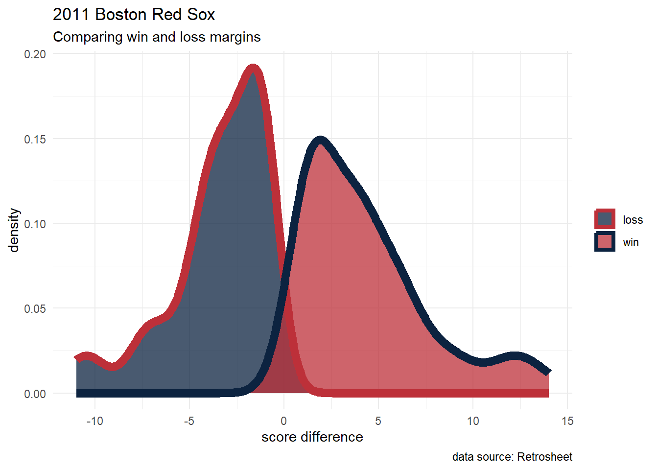

graph code

BOS_2011 |>
  ggplot(aes(x = ScoreDiff)) +
  geom_density(aes(color = W_bool,
                   fill = W_bool),
               alpha = 0.75,
               linewidth = 3) +
  labs(title = "2011 Boston Red Sox",
       subtitle = "Comparing win and loss margins",
       caption = "data source: Retrosheet",
       x = "score difference") +
  scale_color_manual(values = c("#BD3039", "#0C2340")) +
  scale_fill_manual(values = c("#0C2340", "#BD3039")) +
  theme_minimal() +
  theme(legend.position = "right",
        legend.title=element_blank())

The 2011 Red Sox had their victories decided by a larger margin than their losses (4.3 vs -3.5 runs on average), leading to their underperformance of the Pythagorean prediction

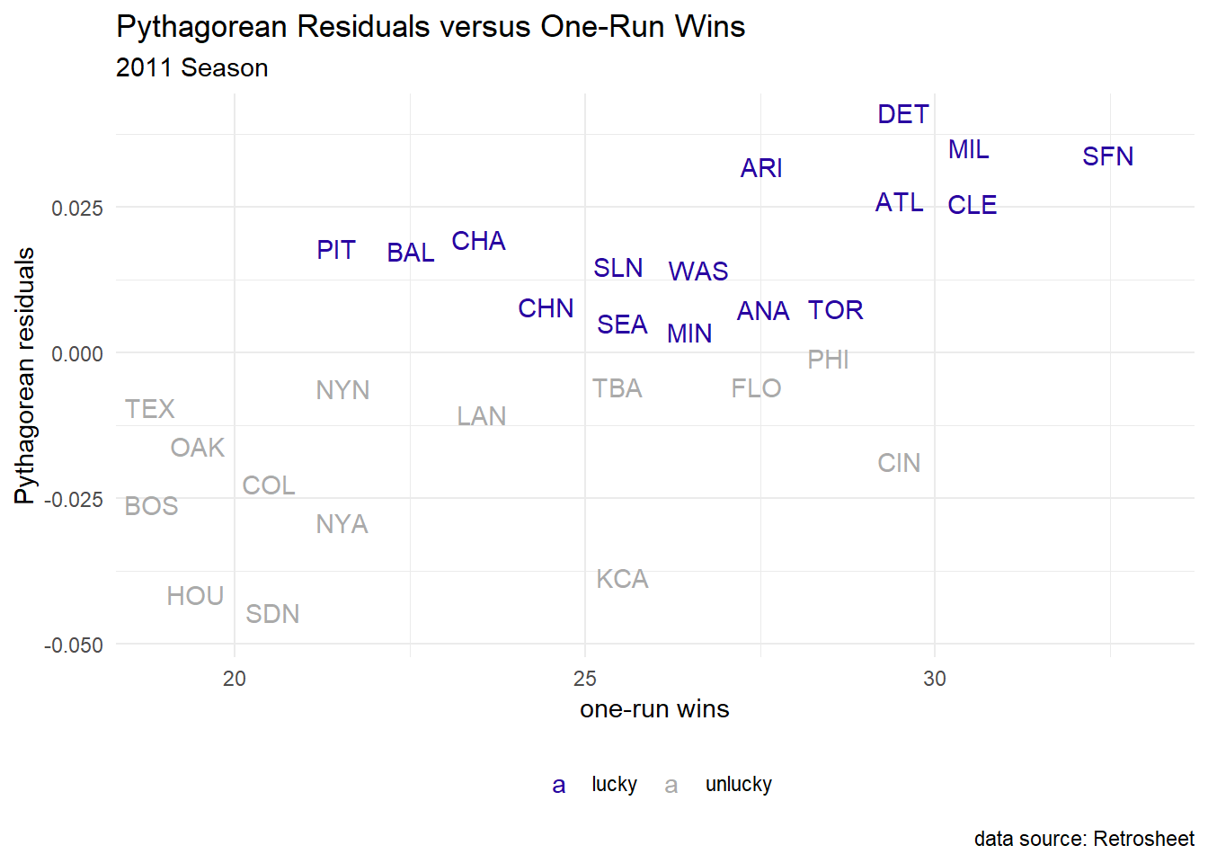
Clutch Performance

Here, we are tracking performance in games won with a difference of just one run.

graph code

one_run_wins <- retro_gl_2011 |>
  select(VisitingTeam, HomeTeam, VisitorRunsScored, HomeRunsScore) |>
  mutate(winner = ifelse(HomeRunsScore > VisitorRunsScored, HomeTeam, VisitingTeam),
    diff = abs(VisitorRunsScored - HomeRunsScore)
  ) |>
  filter(diff == 1) |>
  group_by(winner) |>
  summarize(one_run_w = n())

teams2011 <- ch4_data |>
  filter(yearID == 2011) |>
  mutate(teamID = if_else(teamID == "LAA", "ANA", as.character(teamID))
  ) |>
  inner_join(one_run_wins, by = c("teamID" = "winner"))

teams2011 |>
  mutate(luck = ifelse(resid_pyt > 0, "lucky", "unlucky")) |>
  ggplot(aes(x = one_run_w, y = resid_pyt)) +
  #geom_point() +
  geom_text_repel(aes(color = luck, label = teamID)) + 
  xlab("One run wins") + ylab("Pythagorean residuals") +
  labs(title = "Pythagorean Residuals versus One-Run Wins",
       subtitle = "2011 Season",
       caption = "data source: Retrosheet",
       x = "one-run wins") +
  scale_color_manual(values = c("#2905A1", "#AAAAAA")) +
  theme_minimal() +
  theme(legend.position = "bottom",
        legend.title=element_blank())

Great Relievers

$G R > 50$
$E R A < 2.50$

We obtain summary statistics on the Pythagorean residuals

   Min. 1st Qu.  Median    Mean 3rd Qu.    Max. 
-0.0617 -0.0086  0.0070  0.0078  0.0227  0.0816

Over a 162-game season, a top reliever provides

$0.0078 * 162 \approx 1.2636 wins$

How Many Runs for a Win?

“ten-runs-equal-one-win” rule of thumb

Earlier:

$\hat{W_{pct}} = 0.5 + 0.0006 * R D$

$R D = 0 \to W_{pct} = 0.5$
- Over 162 games: 81 wins
$R D = + 10 \to W_{pct} = 0.506$
- Over 162 games: 82 wins

Calculus

Ralph Caola derived the number of extra runs needed to get an extra win in a more rigorous way using calculus

$W = \frac{G \cdot R^{2}}{R^{2} + R A^{2}}$

\begin{array}{rcl} \frac{\partial W}{\partial R} & = & \frac{\partial}{\partial R} \frac{G \cdot R^{2}}{R^{2} + R A^{2}} \\ = & \frac{2 \cdot G \cdot R \cdot R A^{2}}{(R^{2} + R A^{2})^{2}} \end{array}

calculus in R!

D(expression(G * R ^ 2 / (R ^ 2 + RA ^ 2)), "R")

G * (2 * R)/(R^2 + RA^2) - G * R^2 * (2 * R)/(R^2 + RA^2)^2

Incremental Runs per Win

$I R / W = \frac{(R^{2} + R A^{2})^{2}}{2 \cdot G \cdot R \cdot R A^{2}}$

We can make a user-defined function (and assuming rate statistics “runs per game” and “runs allowed per game” to remove $G$ ):

IR <- function(RS = 5, RA = 5) {
  (RS ^ 2 + RA ^ 2)^2 / (2 * RS * RA ^ 2)
}

With two inputs, we will use a grid search to express different numbers of runs scored and runs allowed.

ir_table <- tidyr::expand_grid(RS = 1:7, RA = 1:7) |>
  mutate(IRW = IR(RS, RA)) |>
  pivot_wider(names_from = RA, values_from = "IRW",
              names_prefix = "RA=")

Incremental runs per win
as posed by Ralph Caola
RS	RA=1	RA=2	RA=3	RA=4	RA=5	RA=6	RA=7
1	2.0	3.1	5.6	9.0	13.5	19.0	25.5
2	6.2	4.0	4.7	6.2	8.4	11.1	14.3
3	16.7	7.0	6.0	6.5	7.7	9.4	11.4
4	36.1	12.5	8.7	8.0	8.4	9.4	10.8
5	67.6	21.0	12.8	10.5	10.0	10.3	11.2
6	114.1	33.3	18.8	14.1	12.4	12.0	12.3
7	178.6	50.2	26.7	18.9	15.6	14.3	14.0

table code

ir_table |>
  gt() |>
  cols_align(align = "center") |>
  data_color(columns = -RS,
             palette = "viridis") |>
  fmt_number(columns = -RS,
             decimals = 1) |>
  tab_header(title = "Incremental runs per win",
             subtitle = "as posed by Ralph Caola")

Exercises

Exercise 4.1

Relationship Between Winning Percentage and Run Differential Across Decades

Section 4.3 used a simple linear model to predict a team’s winning percentage based on its run differential. This model was fit using team data since the 2001 season.

Refit this linear model using data from the seasons 1961–1970, the seasons 1971–1980, the seasons 1981–1990, and the seasons 1991–2000.
Compare across the five decades the predicted winning percentage for a team with a run differential of 10 runs.

Run Differential: +10
over the decades
decade	beta_0	beta_1	RD_10
1910 to 1919	0.49996	0.00076	0.50754
1920 to 1929	0.49999	0.00063	0.50629
1930 to 1939	0.49988	0.00062	0.50605
1940 to 1949	0.49985	0.00066	0.50643
1950 to 1959	0.49997	0.00064	0.50632
1960 to 1969	0.49993	0.00071	0.50704
1970 to 1979	0.50000	0.00064	0.50639
1980 to 1989	0.49993	0.00071	0.50701
1990 to 1999	0.50000	0.00063	0.50632
2000 to 2009	0.49999	0.00062	0.50621
2010 to 2019	0.49999	0.00061	0.50607
2020 to 2023	0.49998	0.00063	0.50624

table code

ch4_1_data <- Teams |>
  select(yearID, teamID, W, L, R, RA) |>
  mutate(RD = R - RA) |>
  mutate(Wpct = W / (W + L))

fit_1910s <- lm(Wpct ~ RD, data = ch4_1_data |> filter(yearID >= 1910 & yearID < 1920))
fit_1920s <- lm(Wpct ~ RD, data = ch4_1_data |> filter(yearID >= 1920 & yearID < 1930))
fit_1930s <- lm(Wpct ~ RD, data = ch4_1_data |> filter(yearID >= 1930 & yearID < 1940))
fit_1940s <- lm(Wpct ~ RD, data = ch4_1_data |> filter(yearID >= 1940 & yearID < 1950))
fit_1950s <- lm(Wpct ~ RD, data = ch4_1_data |> filter(yearID >= 1950 & yearID < 1960))
fit_1960s <- lm(Wpct ~ RD, data = ch4_1_data |> filter(yearID >= 1960 & yearID < 1970))
fit_1970s <- lm(Wpct ~ RD, data = ch4_1_data |> filter(yearID >= 1970 & yearID < 1980))
fit_1980s <- lm(Wpct ~ RD, data = ch4_1_data |> filter(yearID >= 1980 & yearID < 1990))
fit_1990s <- lm(Wpct ~ RD, data = ch4_1_data |> filter(yearID >= 1990 & yearID < 2000))
fit_2000s <- lm(Wpct ~ RD, data = ch4_1_data |> filter(yearID >= 2000 & yearID < 2010))
fit_2010s <- lm(Wpct ~ RD, data = ch4_1_data |> filter(yearID >= 2010 & yearID < 2020))
fit_2020s <- lm(Wpct ~ RD, data = ch4_1_data |> filter(yearID >= 2020))

pred_1910s_R10 <- predict(fit_1910s, newdata = data.frame(RD = 10))
pred_1920s_R10 <- predict(fit_1920s, newdata = data.frame(RD = 10))
pred_1930s_R10 <- predict(fit_1930s, newdata = data.frame(RD = 10))
pred_1940s_R10 <- predict(fit_1940s, newdata = data.frame(RD = 10))
pred_1950s_R10 <- predict(fit_1950s, newdata = data.frame(RD = 10))
pred_1960s_R10 <- predict(fit_1960s, newdata = data.frame(RD = 10))
pred_1970s_R10 <- predict(fit_1970s, newdata = data.frame(RD = 10))
pred_1980s_R10 <- predict(fit_1980s, newdata = data.frame(RD = 10))
pred_1990s_R10 <- predict(fit_1990s, newdata = data.frame(RD = 10))
pred_2000s_R10 <- predict(fit_2000s, newdata = data.frame(RD = 10))
pred_2010s_R10 <- predict(fit_2010s, newdata = data.frame(RD = 10))
pred_2020s_R10 <- predict(fit_2020s, newdata = data.frame(RD = 10))

starts <- seq(1910, 2020, by = 10)
ends   <- c(seq(1919, 2019, by = 10), 2023)
decade <- paste(starts, "to", ends)
beta_0 <- c(
  fit_1910s$coefficients[1],
  fit_1920s$coefficients[1],
  fit_1930s$coefficients[1],
  fit_1940s$coefficients[1],
  fit_1950s$coefficients[1],
  fit_1960s$coefficients[1],
  fit_1970s$coefficients[1],
  fit_1980s$coefficients[1],
  fit_1990s$coefficients[1],
  fit_2000s$coefficients[1],
  fit_2010s$coefficients[1],
  fit_2020s$coefficients[1])
beta_1 <- c(
  fit_1910s$coefficients[2],
  fit_1920s$coefficients[2],
  fit_1930s$coefficients[2],
  fit_1940s$coefficients[2],
  fit_1950s$coefficients[2],
  fit_1960s$coefficients[2],
  fit_1970s$coefficients[2],
  fit_1980s$coefficients[2],
  fit_1990s$coefficients[2],
  fit_2000s$coefficients[2],
  fit_2010s$coefficients[2],
  fit_2020s$coefficients[2])
RD_10 <- c(
  pred_1910s_R10,
  pred_1920s_R10,
  pred_1930s_R10,
  pred_1940s_R10,
  pred_1950s_R10,
  pred_1960s_R10,
  pred_1970s_R10,
  pred_1980s_R10,
  pred_1990s_R10,
  pred_2000s_R10,
  pred_2010s_R10,
  pred_2020s_R10)

df_4_1 <- data.frame(decade, beta_0, beta_1, RD_10)

df_4_1 |>
  gt() |>
  cols_align(align = "center") |>
  fmt_number(columns = -decade,
             decimals = 5) |>
  tab_header(title = "Run Differential: +10",
             subtitle = "over the decades") |>
  tab_style(
    style = list(
      cell_fill(color = "dodgerblue"),
      cell_text(weight = "bold")),
    locations = cells_body(columns = RD_10))

Exercise 4.2

Pythagorean Residuals for Poor and Great Teams in the 19th Century

As baseball was evolving into its modern form, 19th century leagues often featured abysmal teams that did not even succeed in finishing their season, as well as some dominant clubs.

Fit a Pythagorean formula model to the run differential, win-loss data for teams who played in the 19th century.
By inspecting the residual plot of your fitted model from (a), did the great and poor teams in the 19th century do better or worse than one would expect on the basis of their run differentials?

$\hat{W_{pct}} = \frac{R^{1.931}}{R^{1.931} + R A^{1.931}}$

R code

ch4_2_data <- Teams |>
  filter(yearID < 1900) |>
  select(yearID, franchID, W, L, R, RA) |>
  mutate(RD = R - RA) |>
  mutate(Wpct = W / (W + L)) |>
  mutate(logWratio = log(W/L),
         logRratio = log(R/RA))

# handle winless teams!
ch4_2_data$logWratio[ch4_2_data$W == 0] <- -3.1415

pyt_fit <- lm(logWratio ~ 0 + logRratio, data = ch4_2_data)
pyt_fit$coefficients

logRratio 
 1.931166

ch4_2_data <- ch4_2_data |>
  mutate(Wpct_pyt = R^1.931 / (R^1.931 + RA^1.931),
         resid_pyt = Wpct - Wpct_pyt)

1800s Baseball
Best Teams
yearID	franchName	W	L	R	RA	Wpct	Wpct_pyt	resid_pyt	desc
1875	Boston Red Stockings	71	8	831	343	0.8987	0.8467	0.0521	lucky
1884	St. Louis Maroons	94	19	887	429	0.8319	0.8026	0.0293	lucky
1872	Boston Red Stockings	39	8	521	236	0.8298	0.8219	0.0079	lucky
1880	Chicago Cubs	67	17	538	317	0.7976	0.7352	0.0624	lucky
1876	Chicago Cubs	52	14	624	257	0.7879	0.8472	−0.0593	unlucky
1885	Chicago Cubs	87	25	834	470	0.7768	0.7516	0.0251	lucky
1885	San Francisco Giants	85	27	691	370	0.7589	0.7696	−0.0107	unlucky
1871	Philadelphia Athletics	21	7	376	266	0.7500	0.6611	0.0889	lucky
1884	Providence Grays	84	28	665	388	0.7500	0.7389	0.0111	lucky
1874	Boston Red Stockings	52	18	735	415	0.7429	0.7510	−0.0081	unlucky

1800s Baseball
Worst Teams
yearID	franchName	W	L	R	RA	Wpct	Wpct_pyt	resid_pyt	desc
1872	Washington Nationals	0	11	80	190	0.0000	0.1584	−0.1584	unlucky
1873	Baltimore Marylands	0	6	26	152	0.0000	0.0320	−0.0320	unlucky
1875	Brooklyn Atlantics	2	42	132	438	0.0455	0.0898	−0.0443	unlucky
1875	Keokuk Westerns	1	12	45	88	0.0769	0.2150	−0.1381	unlucky
1873	Elizabeth Resolutes	2	21	98	299	0.0870	0.1040	−0.0170	unlucky
1872	Brooklyn Eckfords	3	26	152	413	0.1034	0.1267	−0.0233	unlucky
1884	Wilmington Quicksteps	2	16	35	114	0.1111	0.0928	0.0183	lucky
1899	Cleveland Spiders	20	134	529	1252	0.1299	0.1593	−0.0294	unlucky
1876	Cincinnati Reds	9	56	238	579	0.1385	0.1523	−0.0138	unlucky
1875	Philadelphia Centennials	2	12	70	138	0.1429	0.2124	−0.0695	unlucky

code for tables

ch4_2_data |>
  select(yearID, franchID, W, L, R, RA, Wpct, Wpct_pyt, resid_pyt) |>
  slice_max(n = 10, order_by = Wpct) |>
  inner_join(TeamsFranchises, by = "franchID") |>
  select(yearID, franchName, W, L, R, RA, Wpct, Wpct_pyt, resid_pyt) |>
  mutate(desc = ifelse(resid_pyt > 0, "lucky", "unlucky")) |>
  gt() |>
  cols_align(align = "center") |>
  data_color(columns = desc,
             palette = "viridis",
             reverse = TRUE) |>
  fmt_number(columns = c(Wpct, Wpct_pyt, resid_pyt),
             decimals = 4) |>
  tab_header(title = "1800s Baseball",
             subtitle = "Best Teams") |>
  tab_style(
    style = list(
      cell_fill(color = "dodgerblue"),
      cell_text(weight = "bold")),
    locations = cells_body(columns = Wpct))

ch4_2_data |>
  select(yearID, franchID, W, L, R, RA, Wpct, Wpct_pyt, resid_pyt) |>
  slice_min(n = 10, order_by = Wpct) |>
  inner_join(TeamsFranchises, by = "franchID") |>
  select(yearID, franchName, W, L, R, RA, Wpct, Wpct_pyt, resid_pyt) |>
  mutate(desc = ifelse(resid_pyt > 0, "lucky", "unlucky")) |>
  gt() |>
  cols_align(align = "center") |>
  data_color(columns = desc,
             palette = "viridis",
             reverse = TRUE) |>
  fmt_number(columns = c(Wpct, Wpct_pyt, resid_pyt),
             decimals = 4) |>
  tab_header(title = "1800s Baseball",
             subtitle = "Worst Teams") |>
  tab_style(
    style = list(
      cell_fill(color = "dodgerblue"),
      cell_text(weight = "bold")),
    locations = cells_body(columns = Wpct))